It's Inauguration Week! Let the Fun Begin!
View details for Inauguration Day and access the full schedule of events.
View details for Inauguration Day and access the full schedule of events.
The synchronization of coupled oscillators is a well studied phenomenon. For example, metronomes can be made to synchronize their ticking by putting them on a rocking platform. Similarly, the oscillating magnetic fields of little loops of superconducting wire with a small section removed can also be made to synchronize by driving them with an external magnetic field. Such loops are called rf SQUIDs. Using computer programs and mathematical models, we could see the degree of SQUID synchronization and its resistance to disturbances. For example, and perhaps counterintuitively, we found that the stronger the coupling between the SQUIDs, the more susceptible the system was to falling out of synchronization.
The entrainment of nonlinear oscillators to a driving sinusoidal wave is a subject of much investigation as the behaviors and the mathematics used to describe them are nontrivial. We study an array of one type of nonlinear oscillator called an rf SQUID, or Superconducting QUantum Interference Device, which can be placed within an AC magnetic field that acts as the driving wave. The inductance of each SQUID creates a magnetic field in response, and the resultant flux within each SQUID is tracked as the oscillating quantity. Neighboring SQUIDs are affected by each other’s fields, effectively coupling neighbors. We model the array behavior numerically, which allows us to test a wide range of parameter values. By comparing the amplitudes and phases of the fluxes, we can get a value for the Kuramoto order parameter, a measure of the synchronicity of the oscillations with a value of one indicating perfect synchronization. Preliminary results for the order parameter show that only in the limit of very weak SQUID damping does the value decrease below one as either the frequency of the AC magnetic field or the strength of the SQUID coupling is varied. It is also possible to use Floquet analysis to test the stability of the synchronization by modeling a small perturbation to each SQUID, one at a time, and seeing whether the perturbations shrink or grow over time. We found, through both numerical computation and analytic calculations, that stronger coupling weakened the stability of the synchronization, while the damping of the SQUIDs initially had a positive effect on the stability until the system was critically damped after which further damping decreased stability. The frequency of the external field had no effect on the stability except when very small. We found that the self-inductance of the SQUIDs was inversely proportional to the stability of the synchronization. The next step would be to test the effect of disorder in the critical current values on our findings, as that would be more realistic.
Superconductivity was first identified in 1911by Heike Kamerlingh Onnes after he had managed to liquify helium, bringing it to just a few degrees above absolute zero. Kamerlingh Onnes noticed that when he then used this liquid helium to cool down mercury, its resistance completely disappeared. Because of this lack of resistance, if you created a loop of superconductor and pass a current through it, the supercurrent would persist for at least 105 years, and some estimates predict no decrease in the magnitude of the current for 1010^(10)! Assuming, of course, you could keep the superconductor cool for that long. This would be easier than you might be thinking, as unlike a normal wire a superconductor would not heat up on its own because that heat is caused by the energy loss due to the resistance of the wire.
A radio frequency Superconducting QUantum Interference Device (rf SQUID) is at its base comprised of a loop of superconducting medium. A small section of this loop is removed, but unlike split ring resonators (SSRs), rf SQUIDs have an insulator plugging the capacitive gap, creating a Josephson Junction (JJ). Named after Brian Josephson who accurately predicted their properties in 1963, JJs have some critical supercurrent they can support, based on the geometry of the junction, and as long as the current passing through the JJ is less than the critical current, the current still experiences no resistance even though it is passing through an insulator and not a superconductor.
More pertinent to this project is what happens when the junction current exceeds the critical current. When this happens, it is possible to reimagine the JJ as a resistor, a capacitor and a superconducting shunt in parallel (RCSJ model) and the total current through the junction is equal to the sum of the currents through each of the three paths.
There are two ways to make an rf SQUID have a circulating current. The first is to feed it an input biasing current. The other, which is what we modeled in this project, is to immerse the SQUID in a fluctuating magnetic field such that the flux pierces perpendicular to the plane of the loop. The inductance of the loop then generates a current as described by Faraday's Law. In a wonderful display of feedback, this current creates a reactionary magnetic field, and so the total flux through the center of the loop becomes the sum of the external flux and the resultant screening flux. The total flux oscillates with changes in the supplied magnetic field, and we are interested in these oscillations.
Perhaps the most interesting application of rf SQUIDs is in the fabrication of metamaterials. Metamaterials are artificially manufactured materials assembled from composite materials as opposed to atoms. Picture a diamond, but instead of each point in the lattice being a carbon atom, it is a man-made meta-atom. These meta-atoms are still comprised of atoms, but the overall metamaterial derives its properties from the structuring of the meta-atoms and not from the base elements of the meta-atoms. Through careful designing of the meta-atoms, the resulting metamaterial can have properties unseen in nature.
Some metamaterials have been shown to be capable of are negative indexes of refraction, superlensing with no diffraction limit, and even cloaking. The use of metamaterials in this way is very new, with theory going back to the late 1960s but actual experimentation only picking up in the 21st century. The use of rf SQUIDs in metamaterials dates back less than a decade, and two dimensional arrays of rf SQUIDs to three years ago.This is a hot area of investigation, and there is still a lot of mystery about collective behavior of a SQUID array.
Note: this section refers to a few figures. The meaning of all the symbols are explained, but if you want a concise description to refer to there is one at the bottom of the page or you can click here.
Our focus was on the synchronization capabilities of the rf SQUID array. Because superconductors must be cooled to very low temperatures and once a SQUID has been fabricated it cannot easily be changed, it was simply unfeasible for us do a thorough analysis of the entire parameter space with physical arrays. This is without even mentioning that actually making an array of SQUIDs is as much an art as it is a science and requires special skill. To circumvent these problems, we used computer simulations to model the behavior of a one dimensional SQUID array. This made changing the SQUIDs or the conditions of the experiment as simple as replacing one variable, or even telling the computer to loop through a set of parameters for automation.
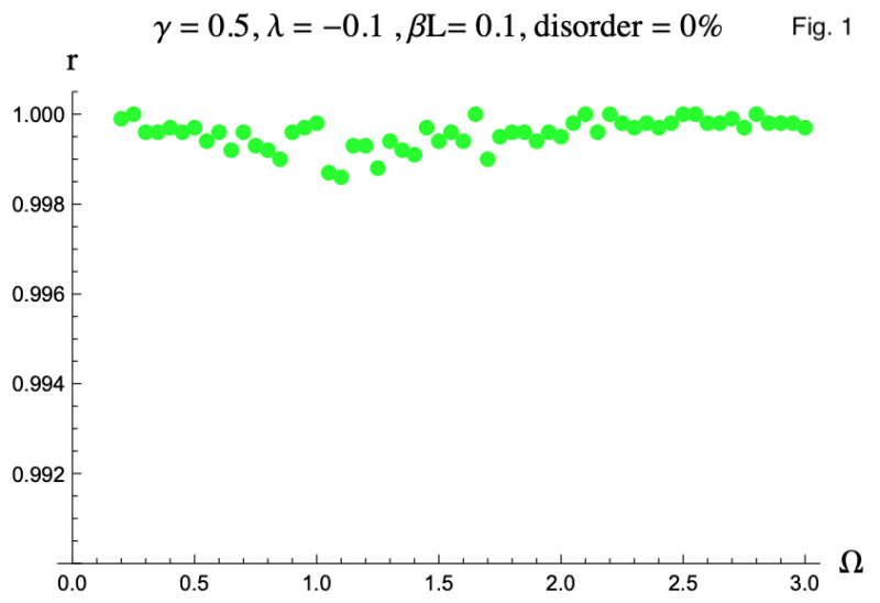
Two quantities in particular interested us. The first was the Kuramoto order parameter, which is a quantification of how in sync a series of oscillators are. The order parameter ranges from 0, no synchronicity, to 1, perfectly in sync. We found that when the SQUIDs are identical, the order parameter did not drift far from 1, which can be seen in Figure 1 (click here to jump to). Figure 1 is a plot of the order parameter (r) against driving flux frequency (Ω). The other symbols are all dimensionless quantities, with 𝛾 referring to the resistive damping of each SQUID, 𝝀 to the inductive coupling of neighboring SQUIDs, and 𝛽L is a product of the inductance of the loop of a SQUID and the critical current of its junction. We found that the more the SQUIDs were damped, the closer the order parameter stayed to 1.
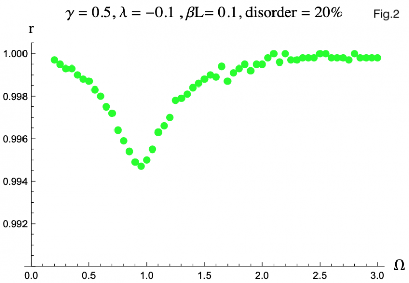
However when we introduced slight differences between the SQUIDs, we noticed a noticeable reduction in the order parameter for frequencies near Ω = 1, as seen in Figure 2. We modeled these differences through disorder in 𝛽L because when physically fabricating an array it would be impossible to ensure each one had a junction exactly the same size, leading to variances in critical currents. With greater damping, the magnitude of the reduction lessened, and its position moved to lower Ω values. The cause of this reduction is likely the small variations in the resonance frequencies of the SQUIDs, which depend on their 𝛽L values. This makes all the SQUIDs oscillate at slightly different phases and amplitudes, the two factors that make up the Kuramoto order parameter.
 The second thing that interested us was the set of Floquet exponents of the system. The Floquet exponents tell you about the stability of the synchronous behavior by predicting if a small disturbance to one of the oscillators would grow over time to destabilize the whole system or if the rest of the oscillators will pull the disturbed one back in sync. If all the Floquet exponents are negative, then perturbations to the system diminish with time; the more negative the Floquet exponents the faster the perturbations will disappear. If, however, even one Floquet exponent is positive then perturbations will grow over time.
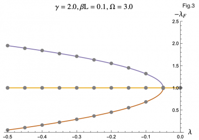
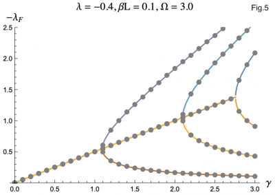
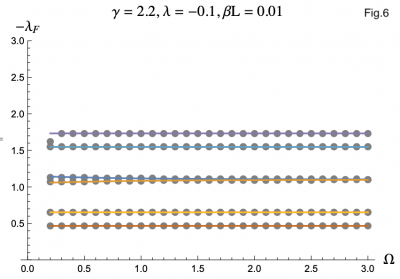
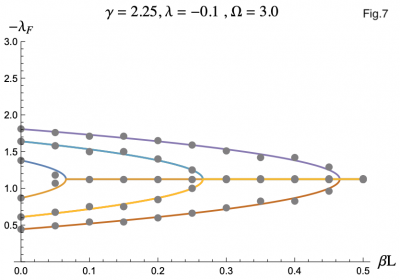
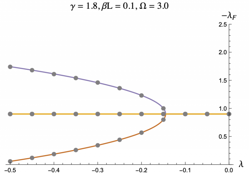
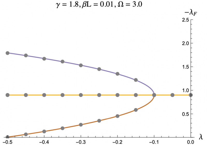
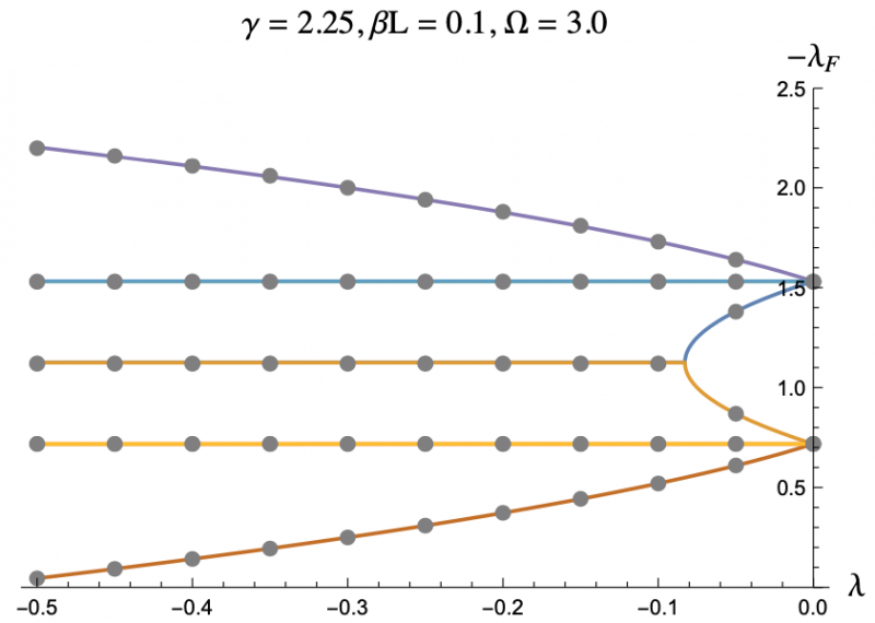
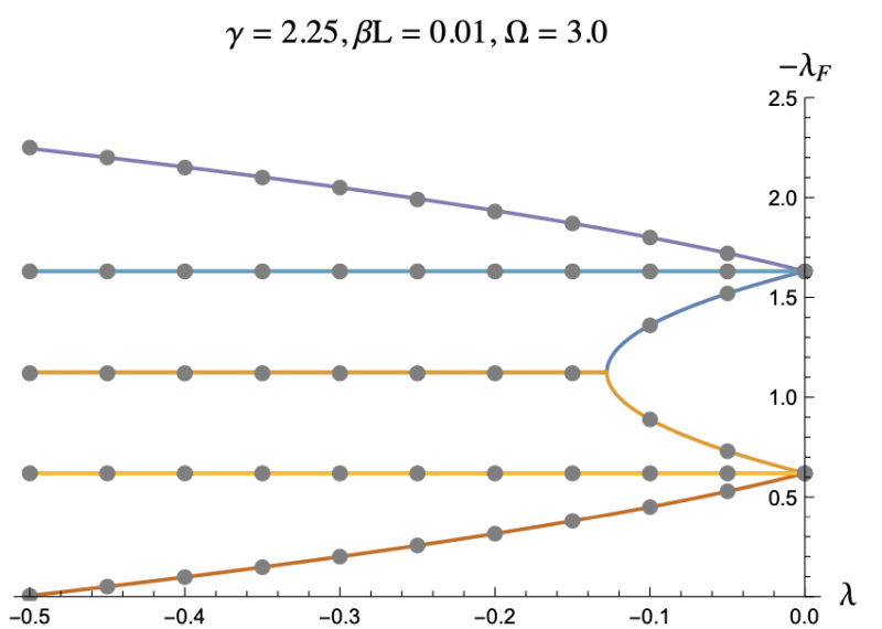
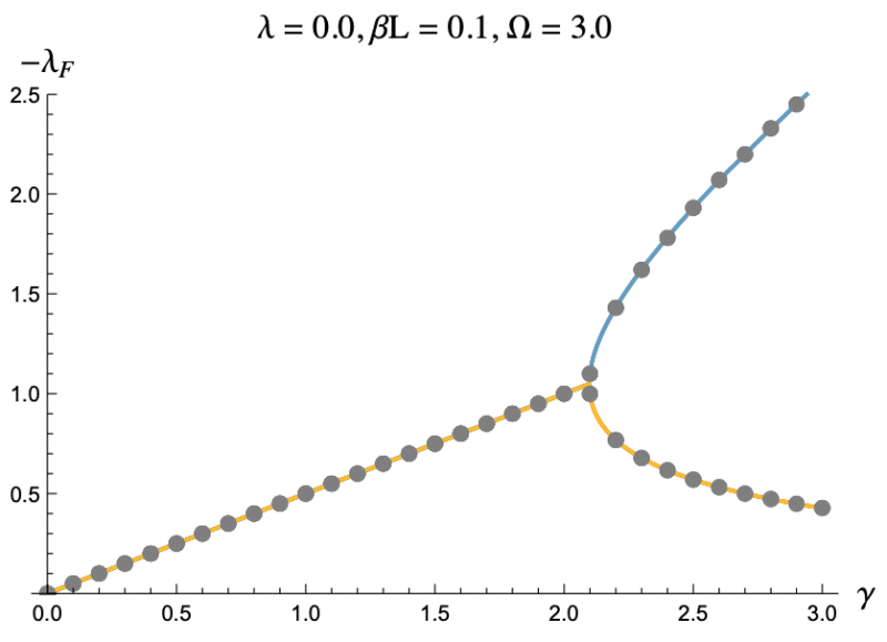
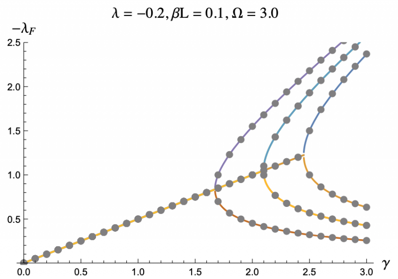
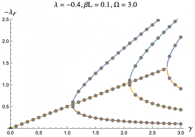
The equation describing the physics of an rf SQUID array is a second order, nonlinear differential equation and can only be solved numerically, hence the computer program. But by using the Poincaré–Lindstedt method of Perturbation Theory, we were able to get an approximate expression for the Floquet exponents with the assumption of Ω > 1. This approximation is represented by the colored lines in Figures 3-7, and lines up perfectly with the results we got from the code represented as grey dots. This allowed us to make predictions and hone in on more interesting regions of parameter space without having to go through the tedious process of repeatedly running the code. The approximation was even reliable for Ω values less than but close to one. We plotted the negative floquet exponents (-𝝀f) versus our four parameters: 𝝀,𝛾,Ω,𝛽L.
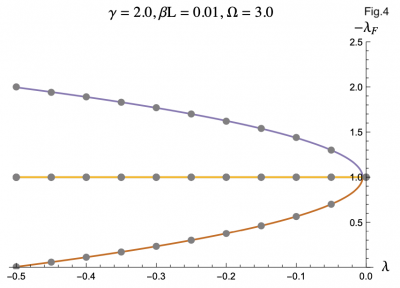
 One thing we noticed immediately is that the higher the magnitude of 𝝀, meaning the more the strongly the SQUIDs were coupled, the weaker the stability of the system became, which can be seen in Figure 3 and Figure 4. This surprised us as we had expected that when coupled more strongly the SQUIDs would have an easier time pulling any rogue members of the array back into synchronization. Instead what seems to be the case is that the SQUIDs are actually synchronizing with the supplied magnetic field, not each other, and are constantly interfering with each others' oscillations. If they are coupled strongly enough, then a disturbance in one SQUID can cause a disastrous chain reaction. This kind of coupling, while unintuitive, does exist, and we have discovered that an array of rf SQUIDs is one such system where this applies. These figures also show you with larger 𝛽L's, the bifurcations start at larger𝝀's.
 The effect of SQUID damping was a bit more complicated, but not surprising. At first, increasing 𝛾 had a beneficial effect on the stability of the array. After some critical 𝛾, however, further damping of the system would cause some of the Floquet exponents to go towards zero, lowering the stability of the system. This behavior, which can be seen in Figure 5, is not unlike the effect of damping on a classical oscillator.
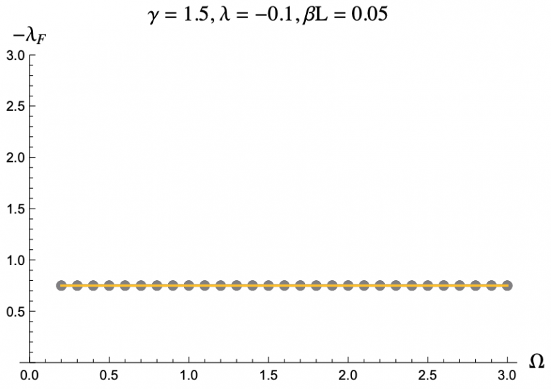
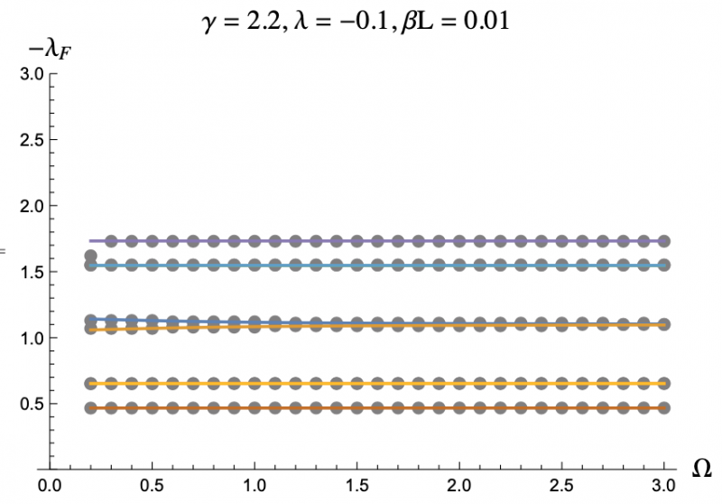
 It turns out Ω has a nearly negligible effect on the Floquet exponents, and only at small values of Ω. Figure 6 depicts a rare case were there is a noticable difference between small and large Ω behavior.
For a reason we have not yet identified, when we plotted -𝝀f versus 𝛽L we didn't get as good agreement as when we varied the other parameters. Here, instead of the grey data points from the code lying directly on top of the colored lines representing the analytic expression, the dots alternated being slightly above and below. Figure 7 is a good example of this. This is still good enough agreement to be within acceptable range, but this behavior suggests that there is something there we have not recognized yet.
Preliminary attempts to identify any effect of 𝛽L disorder on the Floquet exponents were ineffective. It is only when the disorder is centered around a 𝛽L that is a bifurcation point (dependent on the choices for the other parameters) that any real effect can be detected. The effect is also a lot more complicated than the simple dip that the disorder causes in the order parameter because some of the SQUIDs will want to bifurcate the Floquet exponents while the others would not, and the way the conflict is resolved is very sensitive to how the 𝛽L values are distributed around the bifurcation point.
Below I have included some more of the plots that might help you build a better picture of our results. At the bottom is a concise key that defines all the symbols in one place.
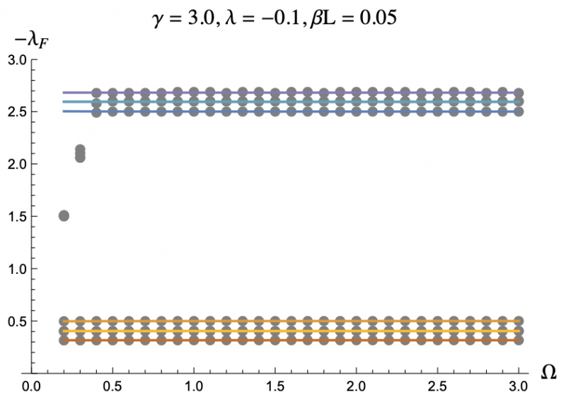
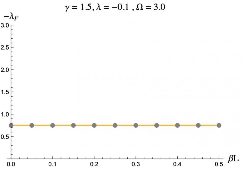
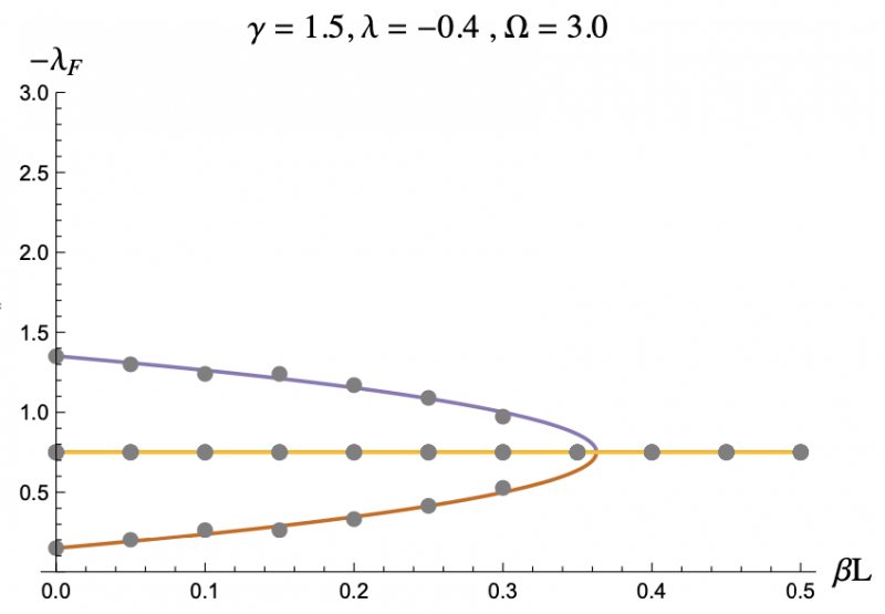
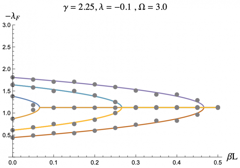
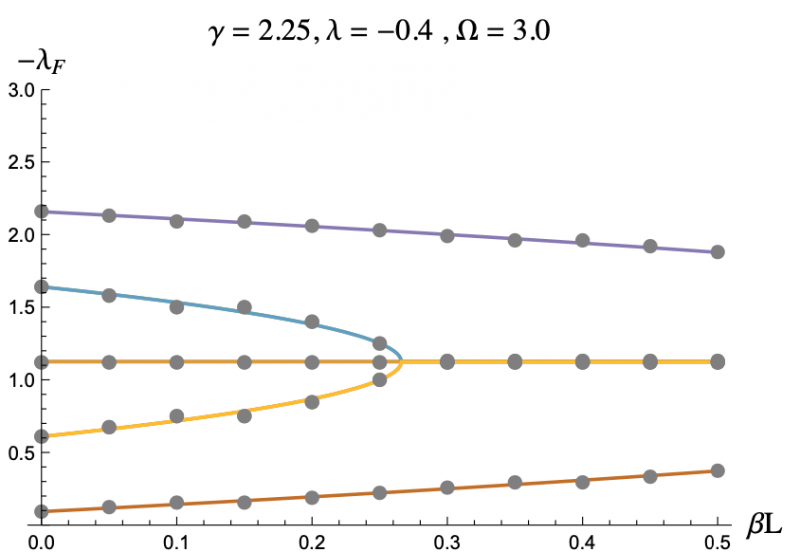
The grey dots refer to the data acquired through code.
The colored lines refer to the analytic expression we approximated.
𝝀f refers to the Floquet exponents.
𝝀 refers to the inductive coupling of the SQUIDs.
𝛾 refers to the resistive damping of the SQUIDs.
Ω refers to the frequency of the driving magnetic field.
𝛽L refers to a product of the inductance of a SQUID and its critical current (the maximum supercurrent allowed across its JJ).